What Are Some Strategies Producers Can Use to Maintain an Elastic Supply?

25 Price Elasticity of Supply

Learning Objectives

1. Explicate the concept of elasticity of supply and its calculation.
2. Explain what information technology means for supply to be price inelastic, unit of measurement price rubberband, cost rubberband, perfectly toll inelastic, and perfectly price elastic.
3. Explain why time is an important determinant of price elasticity of supply.
4. Apply the concept of price elasticity of supply to the labor supply curve.

The elasticity measures encountered so far in this chapter all relate to the demand side of the market. It is also useful to know how responsive quantity supplied is to a change in toll.

Suppose the demand for apartments rises. At that place will be a shortage of apartments at the old level of apartment rents and force per unit area on rents to ascent. All other things unchanged, the more than responsive the quantity of apartments supplied is to changes in monthly rents, the lower the increment in rent required to eliminate the shortage and to bring the market dorsum to equilibrium. Conversely, if quantity supplied is less responsive to toll changes, price volition have to ascent more than to eliminate a shortage caused past an increase in demand.

This is illustrated in Effigy 3.10 "Increase in Apartment Rents Depends on How Responsive Supply Is". Suppose the rent for a typical apartment had been R ₀ and the quantity Q ₀ when the demand curve was D _i and the supply bend was either S ₁ (a supply curve in which quantity supplied is less responsive to price changes) or S _two (a supply bend in which quantity supplied is more than responsive to toll changes). Note that with either supply curve, equilibrium cost and quantity are initially the same. At present suppose that need increases to D ₂, perhaps due to population growth. With supply bend Due south _ane, the price (rent in this case) will rise to R _ane and the quantity of apartments will ascension to Q ₁. If, however, the supply curve had been S ₂, the rent would merely accept to rise to R ₂ to bring the market place back to equilibrium. In improver, the new equilibrium number of apartments would be college at Q ₂. Supply curve Due south ₂ shows greater responsiveness of quantity supplied to price alter than does supply curve S ₁.

Figure 3.x Increment in Apartment Rents Depends on How Responsive Supply Is

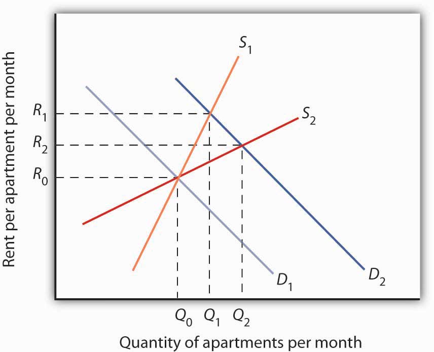
The more responsive the supply of apartments is to changes in price (rent in this case), the less rents ascent when the demand for apartments increases.

Nosotros mensurate the cost elasticity of supply (east_S ) as the ratio of the percentage change in quantity supplied of a good or service to the percentage change in its price, all other things unchanged:

Equation 3.five

[latex]e_S = \frac{ \% \: change \: in \: quantity \: supplied}{ \% \: change \: in \: price}[/latex]

Because price and quantity supplied normally move in the same direction, the cost elasticity of supply is ordinarily positive. The larger the price elasticity of supply, the more responsive the firms that supply the proficient or service are to a cost modify.

Supply is price elastic if the toll elasticity of supply is greater than 1, unit price elastic if it is equal to one, and toll inelastic if information technology is less than ane. A vertical supply bend, every bit shown in Panel (a) of Figure three.11 "Supply Curves and Their Price Elasticities", is perfectly inelastic; its price elasticity of supply is zip. The supply of Beatles' songs is perfectly inelastic because the band no longer exists. A horizontal supply curve, equally shown in Panel (b) of Effigy 3.11 "Supply Curves and Their Price Elasticities", is perfectly elastic; its cost elasticity of supply is infinite. It means that suppliers are willing to supply whatever amount at a sure price.

Figure three.11 Supply Curves and Their Price Elasticities

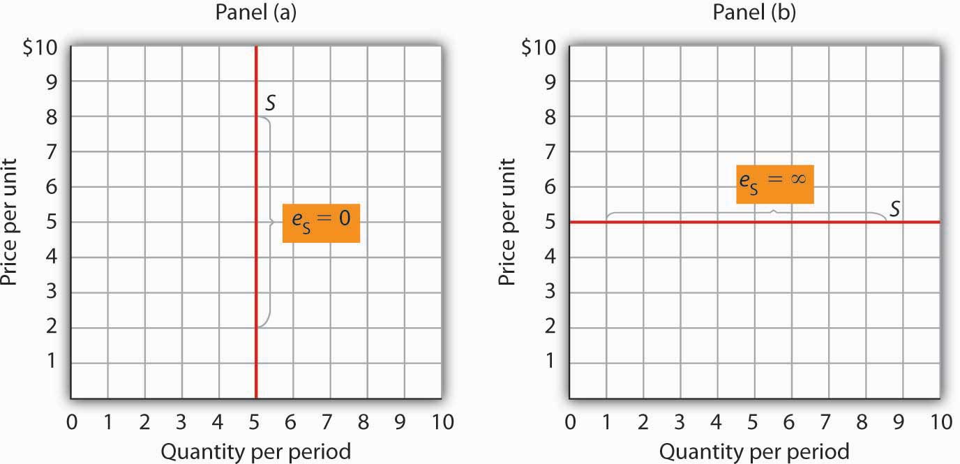
The supply curve in Panel (a) is perfectly inelastic. In Console (b), the supply curve is perfectly rubberband.

Time: An Important Determinant of the Elasticity of Supply

Time plays a very important function in the determination of the price elasticity of supply. Wait again at the effect of rent increases on the supply of apartments. Suppose flat rents in a urban center rise. If we are looking at a supply curve of apartments over a period of a few months, the rent increase is likely to induce apartment owners to rent out a relatively pocket-size number of additional apartments. With the higher rents, flat owners may be more vigorous in reducing their vacancy rates, and, indeed, with more people looking for apartments to rent, this should be fairly easy to attain. Attics and basements are easy to renovate and rent out every bit boosted units. In a short period of fourth dimension, however, the supply response is likely to be adequately modest, implying that the price elasticity of supply is fairly low. A supply curve respective to a short period of time would expect similar Due south ₁ in Figure five.10 "Increase in Apartment Rents Depends on How Responsive Supply Is". It is during such periods that in that location may be calls for hire controls.

If the period of fourth dimension under consideration is a few years rather than a few months, the supply curve is likely to exist much more price elastic. Over time, buildings can exist converted from other uses and new apartment complexes can be congenital. A supply curve corresponding to a longer menstruum of time would expect like S _ii in Figure 5.x "Increase in Apartment Rents Depends on How Responsive Supply Is".

Elasticity of Labor Supply: A Special Application

The concept of cost elasticity of supply can be applied to labor to show how the quantity of labor supplied responds to changes in wages or salaries. What makes this instance interesting is that it has sometimes been found that the measured elasticity is negative, that is, that an increment in the wage rate is associated with a reduction in the quantity of labor supplied.

In most cases, labor supply curves have their normal upward slope: higher wages induce people to work more. For them, having the additional income from working more is preferable to having more than leisure time. All the same, wage increases may pb some people in very highly paid jobs to cut back on the number of hours they piece of work because their incomes are already high and they would rather take more time for leisure activities. In this case, the labor supply curve would have a negative gradient. The reasons for this phenomenon are explained more fully in a later chapter.

This chapter has covered a multifariousness of elasticity measures. All report the caste to which a dependent variable responds to a change in an independent variable. Every bit we accept seen, the caste of this response tin play a critically important office in determining the outcomes of a wide range of economical events. Tabular array 3.2 "Selected Elasticity Estimates"¹ provides examples of some estimates of elasticities.

Table 3.ii Selected Elasticity Estimates

Product	Elasticity	Product	Elasticity	Production	Elasticity
Toll Elasticity of Demand		Cross Cost Elasticity of Demand		Income Elasticity of Demand
Crude oil (U.S.)*	−0.06	Alcohol with respect to price of heroin	−0.05	Speeding citations	−0.26 to −0.33
Gasoline	−0.1	Fuel with respect to price of send	−0.48	Urban Public Trust in French republic and Madrid (respectively)	−0.23; −0.26
Speeding citations	−0.21	Booze with respect to price of food	−0.16	Ground beefiness	−0.197
Cabbage	−0.25	Marijuana with respect to price of heroin (similar for cocaine)	−0.01	Lottery instant game sales in Colorado	−0.06
Cocaine (2 estimates)	−0.28; −1.0	Beer with respect to price of wine distilled liquor (immature drinkers)	0.0	Heroin	−0.00
Alcohol	−0.30	Beer with respect to price of distilled liquor (immature drinkers)	0.0	Marijuana, alcohol, cocaine	+0.00
Peaches	−0.38	Pork with respect to price of poultry	0.06	Potatoes	0.15
Marijuana	−0.four	Pork with respect to price of footing beef	0.23	Food**	0.2
Cigarettes (all smokers; ii estimates)	−0.iv; −0.32	Ground beef with respect to toll of poultry	0.24	Clothing***	0.three
Crude oil (U.S.)**	−0.45	Ground beef with respect to price of pork	0.35	Beer	0.4
Milk (two estimates)	−0.49; −0.63	Coke with respect to toll of Pepsi	0.61	Eggs	0.57
Gasoline (intermediate term)	−0.v	Pepsi with respect to toll of Coke	0.80	Coke	0.60
Soft drinks	−0.55	Local television advert with respect to price of radio advertizement	one.0	Shelter**	0.7
Transportation*	−0.half-dozen	Smokeless tobacco with respect to price of cigarettes (young males)	one.2	Beef (table cuts—not ground)	0.81
Food	−0.7	Price Elasticity of Supply		Oranges	0.83
Beer	−0.7 to −0.9	Physicians (Specialist)	−0.3	Apples	1.32
Cigarettes (teenagers; two estimates)	−0.9 to −one.5	Physicians (Master Care)	0.0	Leisure**	1.4
Heroin	−0.94	Physicians (Immature male)	0.ii	Peaches	1.43
Footing beefiness	−one.0	Physicians (Young female person)	0.five	Health care**	1.half-dozen
Cottage cheese	−1.1	Milk*	0.36	Higher educational activity	1.67
Gasoline**	−ane.5	Milk**	0.5
Coke	−i.71	Child care labor	2
Transportation	−1.9
Pepsi	−2.08
Fresh tomatoes	−2.22
Food**	−2.3
Lettuce	−2.58
Note: *=brusque-run; **=long-run

Key Takeaways

• The price elasticity of supply measures the responsiveness of quantity supplied to changes in toll. It is the pct change in quantity supplied divided past the percentage alter in cost. Information technology is usually positive.
• Supply is price inelastic if the price elasticity of supply is less than 1; it is unit toll elastic if the price elasticity of supply is equal to 1; and it is cost elastic if the price elasticity of supply is greater than 1. A vertical supply curve is said to be perfectly inelastic. A horizontal supply curve is said to be perfectly rubberband.
• The toll elasticity of supply is greater when the length of time under consideration is longer because over time producers have more options for adjusting to the alter in price.
• When applied to labor supply, the price elasticity of supply is usually positive but tin exist negative. If higher wages induce people to work more than, the labor supply curve is upward sloping and the toll elasticity of supply is positive. In some very high-paying professions, the labor supply curve may accept a negative slope, which leads to a negative price elasticity of supply.

Try It!

In the late 1990s, information technology was reported on the news that the high-tech manufacture was worried about being able to find enough workers with estimator-related expertise. Job offers for contempo college graduates with degrees in information science went with high salaries. It was as well reported that more than undergraduates than e'er were majoring in informatics. Compare the price elasticity of supply of calculator scientists at that indicate in time to the cost elasticity of supply of computer scientists over a longer menses of, say, 1999 to 2009.

Instance in Signal: Oil Prices Revisited

WTI Crude Oil Spot price

Recall from our discussion of the dynamics of the earth oil prices before in Chapter 2 that in early 2016, the earth cost of oil vicious to almost $30 per barrel. In this situation, the OPEC countries, which were losing their revenue from oil sales, faced a tough selection: cutting their oil production to prop upwardly the price, equally they've done in the past, or maintain their output and allow the toll go on to fall with the purpose of driving the producers of the more than costly shale oil out of the market. As nosotros could see, OPEC decided non just to become with the latter option, but increase their oil production essentially. What we've learned above about the price elasticities of need and supply volition assistance us ameliorate understand why OPEC made that decision.

Let'due south see what would have happened had OPEC decided to cut its oil production instead of increasing it. Suppose OPEC is making its determination when the price of oil has fallen to $30 and the world pro-duction of oil is 100 one thousand thousand barrels per solar day. OPEC accounts for about 40% of the world oil product, i.due east. produces forty million barrels per day, and then its total revenue from oil is $30×40 million = $1,200 one thousand thousand or $1.2 billion. Will OPEC be able to increase its oil revenue if it reduces its production target past, say, 5%, to boost the price?

Let's starting time consider what will happen in a very short run, when other countries don't have enough time to increase their oil production. Effigy 5.thirteen illustrates this situation. The world market place is initially in equilibrium at point E1, where the toll of oil is $30 per barrel and 100 million barrels per day is supplied. In the very curt run, the supply of oil is practically perfectly inelastic; that is, the supply curve is vertical.

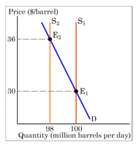
Figure iii.12

If OPEC cuts its oil production past 5% (i.e. by 40 1000000 × 0.05 = 2 million barrels per day), the globe production will decrease from 100 million to 98 million barrels per day. That is, the OPEC'south product cut will shift the supply curve from S1 to S2, so the market will move along the demand bend (D) from the initial equilibrium, E1, to a new equilibrium, E2, where the price is higher.

We can predict what the new price of oil will exist given that the curt-run price elasticity of demand for oil is estimated at −0.1. Since the pct change in quantity is −2% (using the conventional formula, %ΔQ = (98 – 100)/100 = −0.02 or −2%), we can write:

[latex]e_S = \frac{ \% \: change \: in \: quantity \: supplied}{ \% \: change \: in \: cost}[/latex]

[latex]{-0.i} = \frac{ {-2{\%}} }{ \% \: modify \: in \: price}[/latex]

Solving this equation for %ΔP, nosotros get:

-0.1 ten %ΔP = -2%

[latex]{{\%}{\Delta}P} = \frac{ {-two{\%}} }{ {-0.one}}[/latex]

= 20%

That is, the cost rises by $30×0.2 = $6, from $30 to $36.

Since OPEC is now selling 38 one thousand thousand barrels of oil at $36 per barrel, its total revenue is $36×38 million = $i,368 1000000. This is $168 one thousand thousand or xiv% more than the revenue OPEC received before the oil production cutting. Thus, by reducing
its oil product OPEC was able to boost the price of oil, which increased its total revenue from oil sales. This should come equally no surprise. As we've learned in this chapter, when the need is price inelastic, raising the price increases
full revenue. And when the need is very cost inelastic (which is the case here), even small reductions in quantity can lead to substantial price hikes and total revenue gains. This, however, is but true if the competition does not influence the market quantity supplied.

And in the case of the nowadays day's earth market for oil, that could be true in a very short run, but non in a longer run.
Let's see how the world market for oil will reply to OPEC'south production cuts in a longer run, when other countries—including such major world oil producers as the United States and Russian federation—increase their production of oil in response to a college cost. Equally we know, both demand and supply are more cost elastic in the long run than in the short run. Figure 5. fourteen shows what happens if the world supply of oil is still inelastic, but no longer perfectly inelastic (say, ES = 0.two) and the demand for oil becomes less inelastic (say, ED = −0.2).

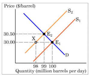
Figure three.13

Now, when OPEC reduces its production of oil past 2 million barrels shifting the earth supply bend from S1 to S2, every bit in Effigy 3.26, other oil producers respond to the initial backlog need for oil and a higher price resulting from it by increasing their production, which partly compensates the OPEC'south reduced supply. The market moves along the supply curve S2 from point Ten to the new equilibrium at indicate E2, where the price of oil is $xxx.50 per barrel and the quantity is 99 one thousand thousand barrels per day. Equally y'all tin can see, considering both need and supply are now less toll inelastic, the price rises only by $one.50 (five%). Will the OPEC'southward total revenue from oil still increase? Annotation first that since other countries increase their oil production while the OPEC countries reduce theirs, the OPEC'due south market share decreases from 40% to 38.4% (equally OPEC is now producing 38 1000000 barrels per day out of the total world product of 99 million barrels per solar day). The OPEC'southward total revenue then is $30.50×38 meg = $1,159 million, which is 3.4% less than its revenue earlier the production cut ($1,200 million). Of course, in an even longer run, when both demand and supply are fifty-fifty more rubberband, OPEC'south oil product cuts to prop up the cost will result in even greater losses of their oil revenues.

Source: Ogloblin, Constantin; Brown, John; King, John; and Levernier, William, "Microeconomics for Business" (2018).Business organisation Administration, Management, and Economics Open Textbooks. 6.

Reply to Try It! Problem

While at a signal in fourth dimension the supply of people with degrees in computer science is very toll inelastic, over time the elasticity should rising. That more students were majoring in information science lends credence to this prediction. As supply becomes more than price rubberband, salaries in this field should rise more slowly.

¹Although close to zero in all cases, the pregnant and positive signs of income elasticity for marijuana, alcohol, and cocaine suggest that they are normal appurtenances, simply meaning and negative signs, in the case of heroin, suggest that heroin is an inferior proficient. Saffer and Chaloupka (cited below) suggest the effects of income for all four substances might exist affected by education. [Other References listed beneath]

References

Adesoji, O. Adelaja, A. "Price Changes, Supply Elasticities, Manufacture Organization, and Dairy Output Distribution," American Journal of Agricultural Economics 73:1 (February 1991):89–102.

Bar-Ilan, A., and Bruce Sacerdote, "The Response of Criminals and Non-Criminals to Fines," Journal of Law and Economics, 47:1 (April 2004): 1–17.

Baye, Chiliad.R., D.W. Jansen, and J.Westward. Lee, "Advertising Effects in Complete Demand Systems," Applied Economic science 24 (1992):1087–1096.

Bhuyan, S., and Rigoberto A. Lopez, "Oligopoly Power in the Food and Tobacco Industries," American Journal of Agricultural Economics 79 (August 1997):1035–1043.

Blau, D. M., "The Supply of Kid Care Labor," Journal of Labor Economics 2(eleven) (April 1993):324–347.

Blundell, R., et al., "What Do We Acquire About Consumer Demand Patterns from Micro Data?", American Economic Review 83(3) (June 1993):570–597.

Bresson, G., Joyce Dargay, Jean-Loup Madre, and Alain Pirotte, "Economic and Structural Determinants of the Demand for French Transport: An Assay on a Panel of French Urban Areas Using Shrinkage Estimators," Transportation Research: Part A 38:four (May 2004): 269–285.

Brester, G. W., and Michael G. Wohlgenant, "Estimating Interrelated Demands for Meats Using New Measures for Ground and Tabular array Cut Beef," American Journal of Agricultural Economics 73 (Nov 1991):1182–1194.

Brown, D. Grand., "The Rising Price of Physicians' Services: A Correction and Extension on Supply," Review of Economics and Statistics 76(2) (May 1994):389–393.

Davis, K. C., and Michael K. Wohlgenant, "Need Elasticities from a Discrete Selection Model: The Natural Christmas Tree Market," Periodical of Agronomical Economic science 75(3) (August 1993):730–738.

Ekelund, R. B., South. Ford, and John D. Jackson. "Are Local TV Markets Divide Markets?" International Periodical of the Economics of Business organization vii:1 (2000): 79–97.

Elzinga, K. G., "Beer," in Walter Adams and James Brock, eds., The Structure of American Industry, 9^th ed. (Englewood Cliffs: Prentice Hall, 1995), pp. 119–151.

Farrelly, M. C., Terry F. Pechacek, and Frank J. Chaloupka; "The Affect of Tobacco Command Program Expenditures on Aggregate Cigarette Sales: 1981–2000," Journal of Wellness Economics 22:5 (September 2003): 843–859.

Fogel, R. W., "Catching Up With the Economy," American Economical Review 89(one) (March, 1999):ane–21.

Gasmi, F., et al., "Econometric Analysis of Collusive Behavior in a Soft-Drinkable Market place," Periodical of Economics and Management Strategy (Summer 1992), pp. 277–311.

Griffin, J. M., and Henry B. Steele, Energy Economics and Policy (New York: Academic Press, 1980), p. 232.

Grossman, M., "A Survey of Economic Models of Addictive Beliefs," Journal of Drug Issues 28:3 (Summer 1998):631–643.

Grossman, M., "Cigarette Taxes," Public Health Reports 112:4 (July/August 1997): 290–297.

Grossman, M., and Henry Saffer, "Beer Taxes, the Legal Drinking Age, and Youth Motor Vehicle Fatalities," Journal of Legal Studies sixteen(two) (June 1987):351–374.

Hansen, A., "The Taxation Incidence of the Colorado State Lottery Instant Game," Public Finance Quarterly 23(3) (July, 1995):385–398.

Heien, D., and Cathy Roheim Wessells, "The Demand for Dairy Products: Structure, Prediction, and Decomposition," American Periodical of Agriculture Economics (May 1988):219–228.

Kleinman, G. A. R., Marijuana: Costs of Abuse, Costs of Control (NY:Greenwood Press, 1989).

Levine, J. M., et al., "The Need for Higher Education in Iii Mid-Atlantic States," New York Economic Review 18 (Fall 1988):3–twenty.

Matas, A., "Demand and Revenue Implications of an Integrated Transport Policy: The Case of Madrid," Transport Reviews, 24:2 (March 2004): 195–217.

Rizzo J. A., and David Blumenthal, "Doc Labor Supply: Do Income Furnishings Matter?" Journal of Health Economics 13(4) (December 1994):433–453.

Ross, H., and Frank J. Chaloupka, "The Effect of Public Policies and Prices on Youth Smoking," Southern Economic Journal 70:4 (Apr 2004): 796–815.

Saffer, H., and Frank Chaloupka, "The Demand for Illicit Drugs," Economic Inquiry 37(3) (July, 1999): 401–411.

Suits, D. B., "Agronomics," in Walter Adams and James Brock, eds., The Structure of American Industry, nine^thursday ed. (Englewood Cliffs: Prentice Hall, , 1995), pp. i–33.

Tauras. J. A., "Public Policy and Smoking Cessation among Immature Adults in the United States," Health Policy, 68:3 (June 2004): 321–332.

coxmencre1945.blogspot.com

Source: https://uw.pressbooks.pub/microman/chapter/3-5-price-elasticity-of-supply/

Share this post